Pages

2/27/07

Want To Protect Your Worksheet Data?

Data in your worksheet can be moved, changed or deleted by any user. If you want to protect important details you will need to lock the cells. No user can edit locked cells without a valid password.

In Excel each cell has the option to lock data using a password. You can lock a cell, a group of cells, rows or columns.

First select all cells in your worksheet. There are two methods to select all the cells.

  1. Press 'Ctrl' key and 'A' Key at a time.
  2. Click ‘Select All’ button. (It should be a gray rectangle in the upper-left corner of a worksheet where the row and column headings meet).
  3. Open Format Cell dialogue box. This also can be done by several ways.
  4. Press 'Ctrl' key and '1' key simultaneously.
  5. Select ‘Cells’ from 'Format' menu
  6. Right clicking mouse, selecting ‘Format Cells’ from pop-up menu.
  7. Click the last tab ‘Protection’ in Format cells dialogue box. (To know more about Format cells dialogue box please read previous postings).
  8. Check the status of locked cells in the ‘Protection’ tab. If the option is checked or enabled then you will need to remove the check mark by clicking on it.
  9. Click on 'Ok' or 'Enter' key on your keyboard.

Now the entire cells in the worksheet are not protected and user can edit any cell and make necessary modifications.

Select data that has to be locked. Open the Format cells dialogue box, click protection tab and enable ‘Lock’.

Locking and unlocking cells does not have any effect until you assign a password to the worksheet.

Click on 'Tools' menu and select ‘Protect sheet’ from ‘Protection’ sub-menu. Excel prompts you to enter a password. Enter your password and click on 'Ok.'

Tips: Passwords can be optional. You can protect your worksheet without a password. This helps when very low level security is enough for your worksheet.

Once you protected the sheet with a password, any cell can be edited except locked cells. To do any modifications in the locked cells you will need to unlock the sheet.

Tips: You can even hide the formulas in the cell from display (viewing through formula bar) by turning on ‘Hide’ option that is just below the ‘Lock’ option.

What would happen if you forget your password?

The worksheet can be unprotected only by entering the correct password. You will not be able to open the worksheet without entering the password.

Also please remember that passwords are case sensitive. So please check ‘Caps lock’ in your keyboard before you enter the password.

Do You Like To Save Your Work Automatically?

While working for long hours incase if your system hanged in between or any application error causes the excel program to close suddenly, the important changes that you made would be lost. It also leads rework.

You can use AutoSave feature in excel to avoid such situation. It is a simple feature that helps you a lot by saving your time by saving workbook automatically.

Where you can use AutoSave effectively?
  • If you are working for long time in a workbook, you can use this feature to avoid data loss by automatically saving your workbook every short time.
  • If the workbook that you are using is shared, this feature updates the status automatically every short interval.

AutoSave is an add-in feature installed with Microsoft Excel. You can find the command Add-Ins on the Tools menu. Click Add-Ins and select ‘Autosave Add-in’ from the list of inbuilt features. Now you can see that Autosave option has been added into Tool menu.

This feature prompts you every 10 minutes whether to save the workbook or not. You can customize the settings by clicking ‘Autosave’ on Tool menu.

A dialogue box appears. You can change the default 10 minutes into any number of minutes (1 to 120 minutes) that you want. By selecting the ‘Save all open workbooks’ you even save the active and inactive workbooks at a time. When the particular interval time reaches excel prompts you whether to save or skip changes. If you want to save changes click save option else skip option to continue your work.

If you do not like to get prompted every time, then you need to turn off ‘Prompt before saving’ option. As a result, whenever the interval time passes Excel saves your work automatically without prompting you each time.

Note: If the add-in is not installed on your computer, you can install it using the ''Add / Remove programs' in Control panel. It is very simple. Click on 'Microsoft Office' or 'Microsoft Excel' in the list and click 'Install / Uninstall' tab. Insert the Installation CD to locate the add-in feature.

Want To Learn How 'COUNT IF' Works?

COUNTIF is the function, which is used to count number of cells in a list that matches a particular condition.

Syntax

=COUNTIF(list,”condition”)

Here list is the range of cells selected and condition can be in the form of arithmetic, text or logical expression.

Find below some of the examples:

In the above picture the range of cells between Row 2 and Row 6 are counted by different expressions.

Arithmetic expressions:

=COUNTIF(B2:B6,”>500”)
Here condition is to count cells that are greater than 500. The range of cells is between B2 and B6. There are two cells (B2 is 780 and B4 is 650) that meet the condition, so COUNTIF function returns 2

Text expression:

=COUNTIF(E2:E6, “Lara”)
Here condition is to count cells that have name Lara. The range of cells is between E2 and E6. Three cells B2, B3 and B5 matches the given condition, so COUNTIF function returns 3

Logical expression:

=COUNTIF(H2:H6, “false”)
Here condition is to count cells that have logical value FALSE. The range of cells is between H2 and H6. Two cells have the matching logical value, so COUNTIF function returns 2.

Intersting posts are yet to come. So keep visiting this blog. :-)

2/26/07

Solve formatting Problem While Importing Data.

TRIM function is used to remove unwanted spaces from text. When importing data from other applications into Excel, there will be lot of spaces formed in between words.

This function helps to remove all the spaces except for single spaces between words.

Syntax for TRIM function

=TRIM(cell reference)

Here cell reference is the cell that has the text to be trimmed. You can either directly type the cell reference or select the cell using your mouse. Remember that only one cell can be selected to perform this function.

Go through the below examples to get a clear idea about the syntax.


Assume that in cell E11 we have the following text.
‘Global       Marketing      Company     -     Tokyo’
=TRIM(E11)

The result we get after using the TRIM function will be the following

‘Global Marketing Company - Tokyo’

2/21/07

Want To See Possible Results Of CONCATENATE Function?

CONCATENATE is a function used to join text in one cell to another. You can find ‘concatenate‘ in paste function dialog box.

Click the ‘Paste Function’ icon in standard tool bar to open function dialog box. Select concatenate function from Text category.

A formula wizard appears in your screen that assists you in building the formula properly. You can drag it in case it covers your working area. Using mouse select the cells from which you want to join text. You can select several cells to form a long chain.

Tip: Use Shift and F3 keys at the same time to open Paste function dialog box.

If you want to type directly the formula please go through the following examples.

=CONCATENATE(G17,G18)

This formula simply joins text in the two cells G17 and G18

=CONCATENATE(G17," ",G18)

This formula joins text in the two cells G17 and G18 with a gap in between.

=CONCATENATE(G18," April’ 05")

This appends text ‘April’ 05’ with the value in G18.

Tips: You can even join texts that are in different cells using a simple method. Go through the previous examples using this easy way.

=G17 & G18

It joins text in the two cells G17 and G18

=G17&" "&G18

It joins text in two cells G17 and G18 with space in between.

=G18&" April' 05"

It appends text April’ 05 with the value in G18

Try yourself and simply your day to day task. This function is very easy to use.

:-)


How To Use 'IF' Function In Spread Sheet

‘IF’ worksheet function is used to check the logical result of a condition and based on that result, directing Excel to be perform an action. Actions include doing some calculation or returning to a value.

The logical result of a condition is either true or false. If the condition is true, the function performs an action. In case if the condition is false, the function performs another action.

The syntax is

=IF(CONDITION, if true what to be executed, if false what to be executed)

Go through some of these examples

=IF(E6>100,E6,””)

Here E6 is the cell, which has some value that may be pure number or result of any formula. If value of E6 is greater than 100 return E6 else return nothing (NULL)

=IF(E6>100,E6,0)

If value of E6 is greater than 100 return E6 else return 0

=IF(E6>100,(E6*5),E6)

If value of E6 is greater than 100 return multiplying E6 with 5, else return 0

=IF(E6>100,(E6*5),(E6*6))

If value of E6 is greater than 100 returns multiplying it with 5, else multiply with 6

=IF((E6+F6)>100,1,0)

If sum of E6 and F6 is greater than 100 return as 1 else 0

Important: Do not leave space within formula. Use commas ( , ) Parentheses correctly.

I hope the above examples helped you to get an idea about 'IF' function. Now, go ahead and try yourself to make some formulas using 'IF'.

Tips: You can even use more than one (up to 8) ‘IF’ function in a single formula.

=IF(E6=1,100,IF(E6=2,200,IF(E6=3,300,IF(E6=4,400,IF(E6=5,500,

IF(E6=6,600,IF(E6=7,700,IF(E6=8,800,0))))))))

Learn How To Summarize Your Data Instantly

If you want to summarize your data fast use Subtotal command to calculate automatically each similar groups and their grand total.

Info: Ensure yourself that your data is labeled and sorted properly before using Subtotal command.

You can find the subtotal command in the Data menu. Excel opens a dialogue box once you click it and displays all the labels in the drop menu ‘At each change in’ in the top of the dialogue box.

Now you need to select one label from the list. The label you selected becomes the Index and other labels are considered as items.

Indexing is done to create a tracking order for calculating subtotal of other items. If there is a change in data in the index Microsoft Excel stops summarizing the values till that point, makes a total and continues the summarizing next similar data.

You can use any one of the FUNCTIONS (COUNT, COUNTA, MAX, MIN, PRODUCT, STDEV, STDEVP, SUM, VAR & VARP) in the dialogue box to find value of items. You can find this option in the middle of the dialogue box.

In the bottom of dialog box all the labels are displayed in the scroll menu ‘Add subtotal to’ and Excel ask you to select one or more than one item that you want to summarize. Selected items are summarized by the FUNCTION based on Indexed label.

The other features in this dialogue box are:

Replace Current Subtotals: In case you summarized a particular field using Subtotals and want to change the index label or summarizing function or items, open subtotal dialogue box make necessary changes in inputs and enable ‘Replace Current Subtotals‘ option. Excel will remove existing subtotal and replaces with the new one based on your input.

Page break between Groups: If data taken to summarize is huge and it is required to take print out for each item, you need to enable the option ‘Page break between Groups’. Excel prepares page break between each group.

Summary below data: This option helps you to get summary details below each summarized item.

Tips: If you want to remove subtotals and get back original data, open subtotal dialogue box and select ‘Remove All’.

The result will have outlines that helps you to overview the data. Outlines help you to expand or collapse the nested items without affecting the data. You can turn off outlines if not required. Open options dialogue box and disable ‘outline symbols’ from windows options in the view tab.

Tips: Press Ctrl key and numerical key 8 at the same time to turn ON or OFF outlines.

Want To Manage WorkBook Easily?

If you aware about Excel file structure, the workbook handling task would become very easy. How a normal textbook has its name and number of pages within it, a Workbook also has a title and number of worksheets within it.

You can see worksheets in the sheet tab, which is just above the status bar. The default number of worksheet in a Workbook is three. Using the following path you can customize the number of worksheets to be opened every time when you create a new file.

Tools => Options => General tab => Sheets in new workbook and change the number.

Inserting worksheets:

To insert an additional worksheet, follow any one of the options below:

  1. Press Shift and F11 key at a time.
  2. Select ‘Insert worksheet’ from Insert Menu
  3. Keep your mouse on sheet tab, which is above status bar and right click the mouse. A pop-up menu appears. Select ‘Insert’ from the pop-up menu. (Recommended option)

Tip: Using this pop-up menu option, you can even insert multiple worksheets. Hold shift key to select many worksheets and select ‘Insert’ from the pop-up menu.

Move or Copy Worksheets

Worksheets can be moved within workbook. It can also be moved to an existing workbook or a new workbook.

To move a worksheet, follow any one of the options below:

  1. Select ‘Move or Copy’ from Edit menu.
  2. Drag the sheet directly into the desired location.
  3. Keep your mouse on sheet tab, which is above status bar and right click the mouse. A pop-up menu appears. Select ‘Move’ from the pop-up menu. (Recommended option)

A dialog box appears now. You need to choose the exact location where you want to move. Use ‘To book’ drop menu if you like to move it to an existing worksheet or a new worksheet.

Tip: To make a similar copy of worksheet please enable the option ‘Create a copy’ in the dialog box.

Info: Always save your workbook before performing this command.

Delete Worksheets

A workbook must have minimum one worksheet. Keeping any one worksheet available in the workbook you can delete one or more number of worksheets.

To delete a worksheet, follow any one of the options below:

  1. Select ‘Delete sheet’ from Edit menu.
  2. Keep your mouse on sheet tab, which is above status bar and right click the mouse. A pop-up menu appears. Select ‘Delete’ from the pop-up menu. (Recommended option)

Tip: Using this pop-up menu option, you can even delete multiple worksheets. Hold your shift key to select many worksheets and select ‘delete’ from the pop-up menu.

Info: Remember deleted sheets will be lost and unrecoverable so always save your workbook before performing deleting operations.

Hide and Unhide Worksheets

You can hide a worksheet if you do not like to keep it in display. You can unhide it whenever you want. Click ‘Format’ Menu, click ‘Sheet’ submenu and find Hide or Unhide options.

Info: Worksheets that are hidden by Visual Basic program cannot be Unhide by this method. We will discuss soon how to unhide a workbook that is made hidden by visual basic program.

2/18/07

Want To Know How To Work With COMMENTS?

While working with Excel it may be necessary to brief at times why the value went up or down. In some places you may want to write some hints about the value for your own reference text. But such references will lead lot of rework while preparing instant reports. Moreover you may not like if they are visible to everyone. Microsoft Excel allows you to create short notes on each cell using a command Comment.

You can find the command in the Insert menu. You can even find it in the pop-up menu. The pop-up menu opens either right clicking your mouse or by pressing Shift key and F10 key at the same time.

Tips: By pressing Shift key and F3 key, you can directly create comment and start writing your note. You can customize the text box size, font, font size and its location. You need to type the text and press enter

You will find a red mark now on the top right corner of the cell. While moving mouse pointer nearer to the cell, Excel displays comments whatever you typed just like the above pictures.

Let us know how to manage these comments now.

To edit a comment use Shift Key and F3 function key at the same time.

You can even do by opening the pop-up menu and selecting ‘Edit Comment’ option to make necessary correction. Select ‘Delete comment’ option to delete the existing comment. Select ‘show comment’ option to keep displaying the comment in the screen.

There is a tool bar specially meant for working with comments. You can activate it by selecting comments from View menu.

Info: Always ensure that comments are not disabled in your Excel environment settings. Otherwise you may not able to see any comments even you create.

You can check the current settings for comments from the following path.

Excel => Tool menu => Options => View Tab => Comments => Comment indicator only.

Be A Master In Using VLOOKUP Function

While working with large number of data it’s really a difficult task and time-consuming process to search data related to a specific field and use it for another purpose. We can use VLOOKUP function in such condition to fetch data related to a particular field from large number of records.

This function can be used effectively in following circumstances.

When an organization has entire details about employees in a worksheet, it is possible to fetch available related data in the worksheet about any employee. Based on employee name or employee ID, VLOOKUP can fetch other existing details like age, date of joining, designation, experience, salary etc.

If a library has the entire details about books, it is possible to fetch existing related data about any book. Based on book name or book ID, VLOOKUP can fetch other existing details like author name, published date, location, member ID to whom the book was issued, issued date etc.

If a Company has entire details about products, it is possible to fetch existing related data about any product. Based on product name product ID, VLOOKUP fetches other details like dimension details, manufacturing details, stock details, price details etc.

The value fetched by VLOOKUP can be effectively used to do another task. If you change the source details, VLOOKUP automatically replaces it over the old value.

Let us discuss VLOOKUP briefly with an example. Please find below picture in which a small part of worksheet is displayed. There are thousands of rows and few columns have details about a product and the range of cells we see in this page is only between A1 to E5.


We are going to fetch price details of a particular product without searching manually and pasting the value.

Syntax for VLOOKUP

=VLOOKUP(KEY FIELD, SOURCE TABLE, COLUMN ID, ACCURACY)

Here key field is the matching data to be searched. Source table is the database. Column ID is the reference column right from the matching key field; Accuracy is the level of accuracy need.

Let us find the price details for a given product in the below example. The format is simple and made with an objective that once we type any Product ID in the cell M9, Excel has to search automatically its price, display the price value and further consider the value to calculate with number of units.

Please look at the syntax here

=VLOOKUP(M9,$A$1:$E$5,4,FALSE)

M9 is the key field to be searched. $A$1:$E$5 is the source table. The number 4 is the column index just right from the key field column. False is the accuracy level.

Here false is meant for accurate matching of M9 in the source table. If true is mentioned then Excel finds a value that is approximate matching to M9. (Choose false by default)

Column Index is based on source table (1=CODE, 2=MODEL, 3=MAKE, 4=PRICE and 5=SIZE). The column index we given 4 is meant for price.

Based on M9 value, the result O9 returns value. Check the right side picture, where the code given is ‘10000288’. Excel searches exact matching word in the source table ($A$1:$E$5) and get the 4th column index value ($4,999.00) in the cell O9.

Fetched value is the price of single unit and P9 is the price of number of units given. You can copy and paste the formula in the below cells to get more product prices.

Tips: Insert $ symbols in source table cell range. This keeps the range of cells unchanged while dragging or pasting into another cell.

Advanced method:

If key field is blank, VLOOKUP returns error message (#N/A). To avoid displaying such messages please change the formula a slightly using IF function. (To know more about IF FUNCTION please go through archives)

Following is the modified syntax

=IF(M9<>0,VLOOKUP(M9,$A1:$E$5,4,FALSE),””)

In case M9 equals zero, IF function returns to blank. Otherwise VLOOKUP will be carried out and excel fetches price value.

=IF(N9<>0,N9*O9,””)

In case the number of product N9 is zero, IF function returns to blank. Else calculates price value for number of products.

2/15/07

Like To Customize Your Sortings?

While working with large data there are some functions that can be effectively used to sort based on specific features within cells. LEN is such a function used to find out the number of characters within a cell.

Below given is the Syntax for LEN Function:

=LEN(Text)

Here Text is the cell reference whose length has to find out. Please go through below examples to know the various possible results.

When a cell reference M24 has value OK

=LEN(M24)

LEN function returns 2 (counted characters O and K)

When a cell reference C2 has value OK!

=LEN(C2)

LEN function returns 3 (counted text including special characters)

When a cell reference P18 has value TYPE A

=LEN(P18)

LEN function returns 6 (counted text including blank spaces)

When a cell reference Y11 has value 120, which is a result of arithmetic operations.

=LEN(Y11)

LEN function returns 3 (counting numbers 1, 2 and 0)

Try any sample from above, you will find it simple.

Want To Perform COUNTIF Function?

COUNTIF is the function, which is used to count number of cells in a list that matches a particular condition.

The Syntax should be the following:

=COUNTIF(list,”condition”)

Here list is the range of cells selected and condition can be in the form of arithmetic, text or logical expression.

Find below some of the examples:

In the above picture, the range of cells between Row 2 and Row 6 are counted by different expressions.

Arithmetic expressions:

=COUNTIF(B2:B6,”>500”)

Here condition is to count cells that are greater than 500. The range of cells is between B2 and B6. There are two cells (B2 is 780 and B4 is 650) that meet the condition, so COUNTIF function returns 2

Text expression:

=COUNTIF(E2:E6, “Lara”)

Here condition is to count cells that have name Lara. The range of cells is between E2 and E6. Three cells B2, B3 and B5 matches the given condition, so COUNTIF function returns 3

Logical expression:

=COUNTIF(H2:H6, “false”)

Here condition is to count cells that have logical value FALSE. The range of cells is between H2 and H6. Two cells have the matching logical value, so COUNTIF function returns 2

Look at the above example and give a try. It is simple!

Do You Want To Print Same Title On Every Page?

Whenever we need to take print out for a long report we observe that Title in the top or left of the report appears only in the first page. We copy them and insert properly to make them appear in all pages. This normal method takes lot of time and leads rework while adjusting margins.

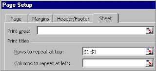
There is an easy way to overcome this problem. Select ‘page setup’ from File menu to open page setup dialogue box. You can find four tabs Page, Margins, Header/Footer and Sheet. Click on ‘Sheet’ tab.


There are two options in the print titles area, which are meant for rows and columns. If your Title is arranged in rows then locate it by using ‘Rows to repeat at top’ option. Excel hides the dialogue box temporarily and prompts your to select the rows. Even if you select one cell, the whole row will be considered for selection. You can even select more than one row to repeat at top every page.

Once you finished selecting rows press enter to return into dialogue box. The range of your selection will be displayed in the range locator. If you want to edit it either you can do directly or select again the title. Ensure that title is being repeated in all sheets before you take print out.

In case if your title is arranged in vertical order then use ‘Columns to repeat at left’ option to locate it.

Tips: If you need to print row and column header of excel sheet, use ‘Row and Column Headings’ option in the same print tab.

I hope that you will find this method very easy to apply in your day to day office work.

2/11/07

Do You Like To Do Copy Paste Instantly?

You can work faster than others if you know about the copying tricks. Though there are many methods available to copy data, try to practice yourself the quickest one.

Following are the methods recommended that save your time.

Press Control key and D key to fill in contents of cells that are above the active cell.

Press Control key and R key to fill in contents of cells that are left to the active cell.

Select any cells and drag towards down (or) left to copy into multiple rows or columns. Hold control key while dragging data to confirm copying action especially for formulas and dates.